A recent question on a website requested for calculating the average of absolute differences for a year-over-data. The question was particularly related to some Economic Values – that was just beyond the level of understanding of a common man, but the point was how we can do it without using a helper column.

The solutions with the helper column are easier to understand and let user device their own solution. But there are times when such helper columns are not welcomes – this was a similar case.

Since that was a data specific to a situation, we have created a dummy table to imitate the actual data, let’s see how we can calculate the average absolute difference.

The Data Table

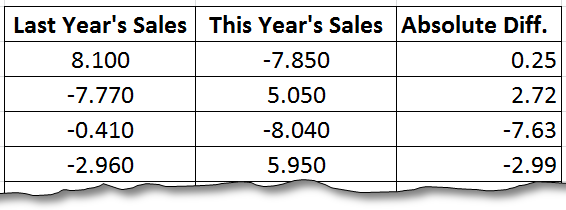
This was the sales data table that was provide with actual question and we can see the helper column on the extreme right. The column uses ABS() function to find the value for negative figures from the table and then subtract the current year’s value from the previous year’s value.  The table returned the following result:

As we are interested in finding it without helper column we will use the following formula:

The formula:

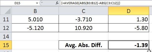
=AVERAGE(ABS(B3:B12)-ABS(C3:C12))

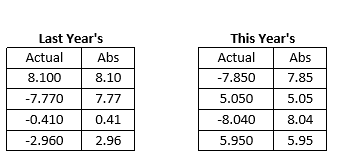
The formula works by taking absolute values for both the years – this removes the negative signs from the data as shown in this table:

Since this is an array formula, ABS(B3:B12)-ABS(C3:C12) will result in taking difference of the respective value for the entire range.

{8.10, 7.77, 0.41, 2.96} - {7.85, 5.05, 8.04, 5.95} = {0.25, 2.72, -7.63, -2.99}

This value is then feed to AVERAGE() function that averages it out to give the answer. The process is simple yet it is a very effective way of simplifying a complex sheet.

The final solution looks like: