Vlookup can be considered as one of the most beneficial functions offered in Microsoft Excel, which has become much useful in data analysis and data processing work.

In Microsoft Excel Vlookup is can be used either with exact match or with multiple criteria. The use of this function is that we can extract data we require from a large set of data sheet.

Someone using Vlookup for the first time may find the syntax to be much complicated which is not the true. Syntax for the vlookup function in excel is as below;

=vlookup(lookup_value,table_array,col_index_num,range_lookup)

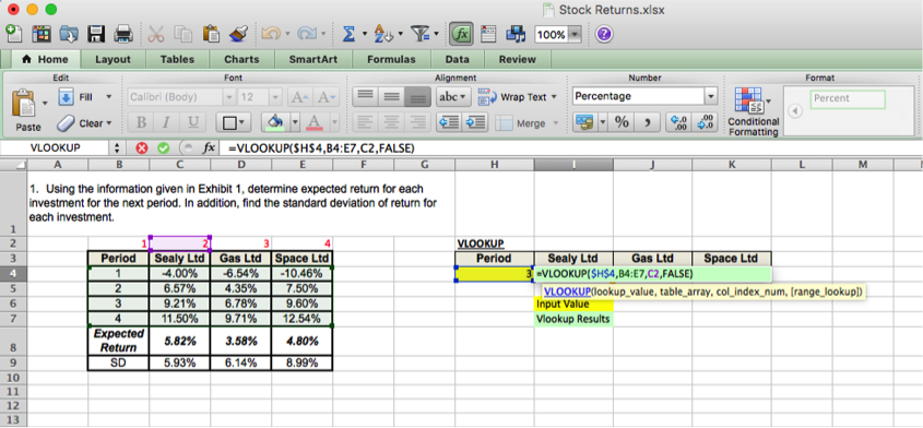
Use of vlookup function with exact much can be demonstrated with the below example.

Steps to follow in using vlookup function:

- First step is to locate the reference table in Excel. It can be on a sheet different from the current worksheet.

In the above figure, reference table is shown towards the left hand side having its four columns labeled in red.

- Then we have to locate the cell into which we need to retrieve data from the reference table.

- Finally, we have to write the formula with correct inputs for the four parameters and hit Enter.

In this example, the reference data is included in the cell range; B4:E7. In the syntax it is referred to as “table_array”. The purpose of the vlookup function is to retrieve a data value from the reference table. In the example, the “lookup_value” is the period of which we want to extract data. It can be 1, 2, 3 or 4.  “col_index_num” is the index of the column from which the data need to be extracted.  Last parameter, “range_lookup” defines whether the vlookup is used to find an exact match or an approximate match.

If the exact match is not found, then the next largest value less than the lookup value is returned when range_lookup is defined as TRUE or omitted.

If the range lookup is defined as FALSE and the exact match is not found, then the value #N/A is returned.